Gaussian Splatting
From Points to Radiance: The Evolution of Gaussian Splatting in Photogrammetry
For decades, the photogrammetric pipeline has remained relatively stable: feature extraction, matching, bundle adjustment, and dense reconstruction. However, as we push toward real-time immersion and digital twins, traditional meshes often fall short—struggling with non-Lambertian surfaces, fine geometries like hair, and computational overhead.
Enter 3D Gaussian Splatting (3DGS). This technique isn’t just a new way to render; it’s a fundamental shift in how we represent captured reality.
The Technical Core: Beyond the Point Cloud
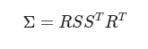
Traditional photogrammetry yields a sparse point cloud. 3DGS takes those points and transforms them into a collection of millions of 3D Gaussians. Each Gaussian is defined by a 3D covariance matrix Σ and a mean position (center) μ.
To keep the representation differentiable and physically meaningful, the covariance matrix is decomposed into a scaling matrix S and a rotation matrix R (represented by a quaternion q):
Each “splat” also carries:
- Opacity (α): Determining how transparent the Gaussian is.
- Spherical Harmonics (SH): Capturing view-dependent color (the “sheen” on a car or the flicker of sunlight on water).
The 3DGS Pipeline for Researchers
The magic of 3DGS is that it leverages the best of photogrammetry to skip the “cold start” problem faced by many neural radiance fields.
- SfM Initialization: You begin with standard photogrammetric software (like COLMAP) to estimate camera poses and generate a sparse point cloud.
- Differentiable Rendering: Unlike NeRFs, which sample points along a ray (a costly process), 3DGS projects these 3D Gaussians into 2D “tiles” on the image plane.
- Adaptive Density Control: During optimization, the system performs “cloning” and “splitting.” If a Gaussian has a high gradient, it’s either split into two smaller ones (if the area is over-reconstructed) or moved (if it’s under-reconstructed).
- Stochastic Gradient Descent: The model minimizes the difference between the rendered splats and the original high-resolution photographs.
Why This Matters for the Digital Twin Era
You likely see the trade-offs in current workflows. 3DGS offers three distinct advantages:
- Training Speed: While a high-quality NeRF might take hours or days to converge, a 3DGS scene can often be “trained” in 20–40 minutes on a single consumer GPU.
- Real-Time Inference: Because the rendering is essentially specialized rasterization, we can achieve 100+ FPS at 1080p resolution.
- Geometric Fidelity: By using the SfM point cloud as a prior, we ensure the spatial coordinates remain grounded in the physical reality of the sensors.
Conclusion: A New Standard?
We are moving away from the era of “hollow” meshes draped in flat textures. We are entering an era of volumetric probability. For researchers in photogrammetry, 3DGS isn’t a replacement for our foundational principles—it is the ultimate refinement of them.